Training a deep learning model for object detection requires a blend of efficient tools, robust datasets, and an understanding of hyperparameters. Ultralytics’ YOLO (You Only Look Once) series has emerged as a favorite in the machine learning community, offering a streamlined approach to object detection tasks.
This blog serves as a complete guide to training YOLO models with Ultralytics, diving deeper into its functionalities, features, and use cases.
Introduction to YOLO Model Training
YOLO models have revolutionized real-time object detection with their speed and accuracy. Unlike traditional methods that require multiple stages for detecting and classifying objects, YOLO performs both tasks in a single forward pass. This makes it a game-changer for applications demanding high-speed object detection, such as autonomous vehicles, surveillance systems, and augmented reality.
The latest iterations, including Ultralytics YOLOv11, are optimized for both versatility and efficiency. These models introduce advanced features, such as multi-scale detection and enhanced augmentation techniques, enabling superior performance across diverse datasets and tasks. Whether you’re a seasoned data scientist or a beginner looking to train your first model, YOLO’s training mode is designed to meet your needs.
Training involves feeding annotated datasets into the model and optimizing parameters to enhance performance. With Ultralytics YOLO, you can train on a variety of datasets—from widely available ones like COCO and ImageNet to your custom datasets tailored to niche applications.
Key benefits of YOLO’s training mode include:
- High Efficiency: Seamless GPU utilization, whether on single or multi-GPU setups.
- Flexibility: Train with hyperparameters tailored to your dataset and goals.
- Ease of Use: Intuitive CLI and Python APIs simplify the training workflow.
By leveraging these benefits, users can build models capable of detecting and classifying objects with remarkable speed and precision.
Key Features of YOLO Training Mode
Ultralytics YOLO’s training mode comes packed with features that streamline the training process:
1. Automatic Dataset
Management YOLO can automatically download and configure popular datasets like COCO, VOC, and ImageNet on first use. This eliminates the hassle of manual setup.
2. Multi-GPU Support
Harness the power of multiple GPUs to accelerate training. Simply specify the GPU IDs to distribute the workload efficiently.
3. Hyperparameter Configuration
Fine-tune performance with an extensive range of customizable hyperparameters, such as learning rate, momentum, and weight decay. These parameters can be adjusted via YAML files or CLI commands.
4. Real-Time Monitoring
Visualize training metrics, loss functions, and other performance indicators in real-time. This allows for better insights into the model’s learning process.
5. Apple Silicon
Optimization Ultralytics YOLO supports training on Apple silicon devices (e.g., M1, M2 chips) via the Metal Performance Shaders (MPS) framework, ensuring efficiency across diverse hardware platforms.
6. Resume Training
Interrupted training sessions can be resumed seamlessly, loading previous weights, optimizer states, and epoch numbers. This feature is particularly valuable for long training runs or when experiments require incremental updates.
Preparing for YOLO Model Training
Successful model training starts with proper preparation. Below are detailed steps to set up your YOLO environment:
1. YOLO Installation:
Begin by installing the Ultralytics YOLO package. It is highly recommended to use a virtual environment to avoid conflicts with other libraries. Installation can be done using pip:
pip install ultralyticsAfter installation, ensure that the dependencies, such as PyTorch, are correctly set up.
2. Dataset Preparation:
The quality and structure of your dataset play a pivotal role in training. YOLO supports both standard datasets like COCO and custom datasets. For custom datasets, ensure that annotations are in YOLO format, specifying bounding box coordinates and corresponding class labels. Tools like LabelImg can assist in creating annotations.
3. Hardware Setup:
YOLO training can be resource-intensive. While it supports CPUs, training on GPUs or Apple silicon chips significantly accelerates the process. Ensure that your hardware is configured with the necessary drivers, such as CUDA for NVIDIA GPUs or Metal for macOS devices.
Usage Examples for YOLO Training
Practical examples help bridge the gap between theory and application. Here’s how you can use YOLO for different training scenarios:
Basic Training Example
Train a YOLOv11 model on the COCO8 dataset for 100 epochs with an image size of 640:
from ultralytics import YOLO

# Load a pretrained model
model = YOLO("yolo11n.pt")

# Train the model
results = model.train(data="coco8.yaml", epochs=100, imgsz=640)
Alternatively, use the CLI for a quick command-line approach:
yolo train data=coco8.yaml epochs=100 imgsz=640Multi-GPU Training
For setups with multiple GPUs, specify the devices to distribute the workload. This is ideal for training on large datasets:
from ultralytics import YOLO

# Load the model
model = YOLO("yolo11n.pt")

# Train with two GPUs
results = model.train(data="coco8.yaml", epochs=100, imgsz=640, device=[0, 1])
Training on Apple Silicon
With macOS devices gaining popularity, YOLO supports training on Apple’s silicon chips using MPS. Here’s an example:
from ultralytics import YOLO

# Load the model
model = YOLO("yolo11n.pt")

# Train with MPS
results = model.train(data="coco8.yaml", epochs=100, imgsz=640, device="mps")
Resume Interrupted Training
When training is interrupted, you can resume it using a saved checkpoint. This saves resources and avoids starting from scratch:
from ultralytics import YOLO

# Load the partially trained model
model = YOLO("path/to/last.pt")

# Resume training
results = model.train(resume=True)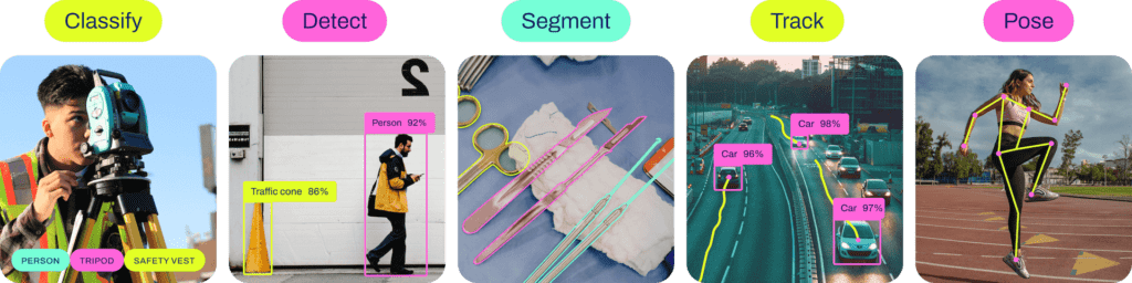
Full Project: End-to-End YOLO Training Example
To illustrate the process of training a YOLO model, let’s walk through an end-to-end project:
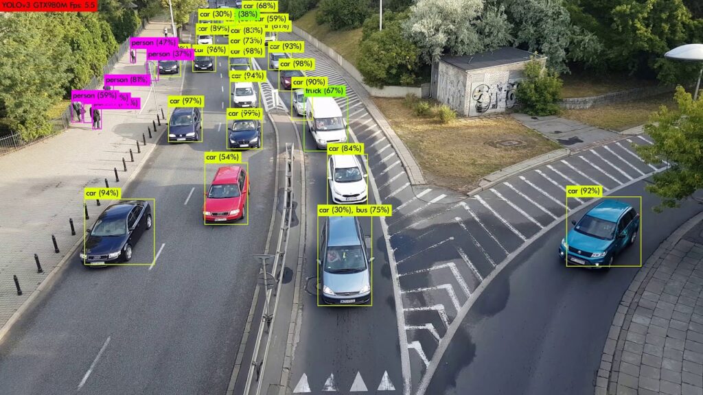
1. Project Overview
In this project, we will train a YOLO model to detect vehicles in traffic images. The dataset consists of annotated images with bounding boxes for cars, trucks, and motorcycles.
2. Step-by-Step Workflow
Dataset Preparation:
- Download the dataset containing traffic images.
- Use annotation tools like LabelImg to label objects in the images and save the labels in YOLO format.
- Organize the dataset into
train,val, andtestdirectories.
Example directory structure:
dataset/
├── train/
│   ├── images/
│   ├── labels/
├── val/
│   ├── images/
│   ├── labels/
├── test/
│   ├── images/
│   ├── labels/
2. Environment Setup:
- Install YOLO using pip:
pip install ultralytics- Verify that GPU or MPS acceleration is configured properly.
3. Model Configuration:
- Choose a YOLO model architecture, such as
yolo11n.yamlfor a lightweight model oryolo11x.yamlfor a more robust model. - Create a custom dataset configuration file (e.g.,
traffic.yaml):
- Choose a YOLO model architecture, such as
train: dataset/train/images
val: dataset/val/images
nc: 3
names: ['car', 'truck', 'motorcycle']
4. Training: Train the YOLO model using the following Python script:
from ultralytics import YOLO
model = YOLO("yolo11n.yaml")

# Train the modelfrom ultralytics import YOLO

# Load a pretrained model
results = model.train(data="traffic.yaml", epochs=50, imgsz=640, batch=16)
Alternatively, use the CLI:
yolo train data=traffic.yaml epochs=50 imgsz=640 batch=165. Validation: Evaluate the model’s performance on the validation set:
metrics = model.val()
print(metrics)
6. Inference: Run inference on test images to visualize results:
results = model.predict(source="dataset/test/images")
results.save()
This will save the output images with bounding boxes to the runs/predict directory.
7. Logging and Monitoring: Use TensorBoard or Comet to log metrics and visualize results:
tensorboard --logdir runs8. Model Export: Export the trained model for deployment:
model.export(format="onnx")The exported model can be used for deployment in applications such as web servers or mobile devices.
Results
Upon completing the training process, the model should be able to accurately detect vehicles in traffic images. Use the validation metrics (e.g., mAP) to assess its performance.
Advanced Training Settings
YOLO models offer a wide range of adjustable settings for fine-tuning:
| Argument | Type | Default | Description |
|---|---|---|---|
| model | str | None | Specifies the model file for training (.pt or .yaml). |
| data | str | None | Path to the dataset configuration file (e.g., coco8.yaml). |
| epochs | int | 100 | Total number of training epochs. |
| batch | int | 16 | Batch size: fixed, auto (60% GPU memory), or custom fraction. |
| imgsz | int/list | 640 | Target image size for training. |
| save | bool | True | Enables saving of training checkpoints and final model weights. |
| device | int/str/list | None | Computational device(s) for training (e.g., GPU IDs, ‘cpu’, ‘mps’). |
| optimizer | str | ‘auto’ | Choice of optimizer: SGD, Adam, AdamW, etc. |
| pretrained | bool/str | True | Start training from a pretrained model (boolean or model path). |
| lr0 | float | 0.01 | Initial learning rate. |
| momentum | float | 0.937 | Momentum factor for optimizers. |
| weight_decay | float | 0.0005 | L2 regularization term to prevent overfitting. |
Augmentation Settings and Hyperparameters
Augmentation techniques play a pivotal role in improving model generalization by introducing variability in training data. Here’s a detailed overview of augmentation arguments supported by YOLO:
| Argument | Type | Default | Range | Description |
|---|---|---|---|---|
| hsv_h | float | 0.015 | 0.0 – 1.0 | Adjusts image hue for color variability. |
| hsv_s | float | 0.7 | 0.0 – 1.0 | Alters saturation for environmental simulation. |
| hsv_v | float | 0.4 | 0.0 – 1.0 | Modifies brightness for lighting conditions. |
| degrees | float | 0.0 | -180 – 180 | Rotates images to improve orientation robustness. |
| translate | float | 0.1 | 0.0 – 1.0 | Translates images to detect partial objects. |
| scale | float | 0.5 | >= 0.0 | Scales images for object size variability. |
| mosaic | float | 1.0 | 0.0 – 1.0 | Combines multiple images for scene complexity. |
| mixup | float | 0.0 | 0.0 – 1.0 | Blends images to generalize better. |
| flipud | float | 0.0 | 0.0 – 1.0 | Flips images upside down for variability. |
| fliplr | float | 0.5 | 0.0 – 1.0 | Flips images left-to-right for symmetry learning. |
Experimenting with these augmentations can lead to significant improvements in model robustness, especially in real-world scenarios with diverse environmental conditions.
Logging and Monitoring
To track your training progress effectively, YOLO integrates with popular logging platforms:
- Comet: Monitor real-time metrics, visualize hyperparameters, and compare experiments.
- ClearML: Manage experiments, share resources, and ensure reproducibility in team environments.
- TensorBoard: Generate interactive plots, including loss curves, accuracy trends, and visualizations of predictions.
Setting up logging is straightforward. For example, you can initialize TensorBoard using the following CLI command:
tensorboard --logdir runsBy leveraging these tools, users can gain actionable insights into their training processes, identify bottlenecks, and refine their models.
Conclusion
Ultralytics YOLO simplifies the complexities of training deep learning models while offering powerful customization options. With features like multi-GPU support, real-time monitoring, and seamless resumption, it’s an invaluable tool for developers and researchers alike.
Whether you’re building a robust object detection system or experimenting with custom datasets, YOLO provides the scalability and flexibility needed to achieve your goals. Start training today and experience the capabilities of YOLO firsthand!