Introduction
Fine-tuning a YOLO model is a targeted effort to adapt powerful, pretrained detectors to a specific domain. The hard part is not the network. It is getting the right labelled data, at scale, with repeatable quality. An automated data-labeling pipeline combines model-assisted prelabels, active learning, pseudo-labeling, synthetic data and human verification to deliver that data quickly and cheaply. This guide shows why that pipeline matters, how its stages fit together, and which controls and metrics keep the loop reliable so you can move from a small seed dataset to a production-ready detector with predictable cost and measurable gains.
Target audience and assumptions
This guide assumes:
You use YOLO (v8+ or similar Ultralytics family).
You have access to modest GPU resources (1–8 GPUs).
You can run a labeling UI with prelabel ingestion (CVAT, Label Studio, Roboflow, Supervisely).
You aim for production deployment on cloud or edge.
End-to-end pipeline (high level)
Data ingestion: cameras, mobile, recorded video, public datasets, client uploads.
Preprocess: frame extraction, deduplication, scene grouping, metadata capture.
Prelabel: run a baseline detector to create model suggestions.
Human-in-the-loop: annotators correct predictions.
Active learning: select most informative images for human review.
Pseudo-labeling: teacher model labels high-confidence unlabeled images.
Combine, curate, augment, and convert to YOLO/COCO.
Fine-tune model. Track experiments.
Export, optimize, deploy. Monitor and retrain.
Design each stage for automation via API hooks and version control for datasets and specs.
Data collection and organization
Inputs and signals to collect for every file:
source id, timestamp, camera metadata, scene id, originating video id, uploader id.
label metadata: annotator id, review pass, annotation confidence, label source (human/pseudo/prelabel/synthetic).
Store provenance. Use scene/video grouping to create train/val splits that avoid leakage.
Target datasets:
Seed: 500–2,000 diverse images with human labels (task dependant).
Scaling pool: 10k–100k+ unlabeled frames for pseudo/AL.
Validation: 500–2,000 strictly human-verified images. Never mix pseudo labels into validation.

Label ontology and specification
Keep class set minimal and precise. Avoid overlapping classes.
Produce a short spec: inclusion rules, occlusion thresholds, truncated objects, small object policy. Include 10–20 exemplar images per rule.
Version the spec and require sign-off before mass labeling.
Track label lineage in a lightweight DB or metadata store.
Pre-labeling (model-assisted)
Why: speeds annotators by 2–10x. How:
Run a baseline YOLO (pretrained) across unlabeled pool. Save predictions in standard format (.txt or COCO JSON).
Import predictions as an annotation layer in UI. Mark bounding boxes with prediction confidence.
Present annotators only images above a minimum score threshold or with predicted classes absent in dataset to increase yield.
Practical command (Ultralytics):
yolo detect predict model=yolov8n.pt source=/data/pool imgsz=640 conf=0.15 save=True
Adjust conf to control annotation effort. See Ultralytics fine-tuning docs for details.
Human-in-the-loop workflow and QA
Workflow:
Pull top-K pre-labeled images into annotation UI.
Present predicted boxes editable by annotator. Show model confidence.
Enforce QA review on a stratified sample. Require second reviewer on disagreement.
Flag images with ambiguous cases for specialist review.
Quality controls:
Inter-annotator agreement tracking.
Random audit sampling.
Automatic bounding-box sanity checks.
Log QA metrics and use them in dataset weighting.
Active learning: selection strategies
Active learning reduces labeling needs by focusing human effort. Use a hybrid selection score:
Selection score = α·uncertainty + β·novelty + γ·diversity
Where:
uncertainty = 1 − max_class_confidence across detections.
novelty = distance in feature space from labeled set (use backbone features).
diversity = clustering score to avoid redundant images.
Common acquisition functions:
Uncertainty sampling (low confidence).
Margin sampling (difference between top two class scores).
Core-set selection (max coverage).
Density-weighted uncertainty (prioritize uncertain images in dense regions).
Recent surveys on active learning show systematic gains and strong sample efficiency improvements. Use ensembles or MC-Dropout for improved uncertainty estimates.
Pseudo-labeling and semi-supervised expansion
Pseudo-labeling lets you expand labeled data cheaply. Risks: noisy boxes hurt learning. Controls:
Teacher strength: prefer a high-quality teacher model (larger backbone or ensemble).
Dual thresholds:
classification_confidence ≥ T_cls (e.g., 0.9).
localization_quality ≥ T_loc (e.g., IoU proxy or center-variance metric).
Weighting: add pseudo samples with lower loss weight
w_pseudo(e.g., 0.1–0.5) or use sample reweighting by teacher confidence.Filtering: apply density-guided or score-consistency filters to remove dense false positives.
Consistency training: augment pseudo examples and enforce stable predictions (consistency loss).
Seminal methods like PseCo and followups detail localization-aware pseudo labels and consistency training. These approaches improve pseudo-label reliability and downstream performance.
Synthetic data and domain randomization
When real data is rare or dangerous to collect, generate synthetic images. Best practices:
Use domain randomization: vary lighting, textures, backgrounds, camera pose, noise, and occlusion.
Mix synthetic and real: pretrain on synthetic, then fine-tune on small real set.
Validate on held-out real validation set. Synthetic validation metrics often overestimate real performance; always check on real data. Recent studies in manufacturing and robotics confirm these tradeoffs.
Tools: Blender+Python, Unity Perception, NVIDIA Omniverse Replicator. Save segmentation/mask/instance metadata for downstream tasks.
Augmentation policy (practical)
YOLO benefits from on-the-fly strong augmentation early in training, and reduced augmentation in final passes.
Suggested phased policy:
Phase 1 (warmup, epochs 0–20): aggressive augment. Mosaic, MixUp, random scale, color jitter, blur, JPEG corruption.
Phase 2 (mid training, epochs 21–60): moderate augment. Keep Mosaic but lower probability.
Phase 3 (final fine-tune, last 10–20% epochs): minimal augment to let model settle.
Notes:
Mosaic helps small object learning but may introduce unnatural context. Reduce mosaic probability in final phases.
Use CutMix or copy-paste to balance rare classes.
Do not augment validation or test splits.
Ultralytics docs include augmentation specifics and recommended settings.
YOLO fine-tuning recipes (detailed)
Choose starting model based on latency/accuracy tradeoff:
Iteration / prototyping:
yolov8n(nano) oryolov8s(small).Production:
yolov8moryolov8l/xdepending on target.
Standard recipe:
Prepare
data.yaml:
					train: /data/train/images
val: /data/val/images
nc: <num_classes>
names: ['class0','class1',...]
2. Stage 1 — head only:
yolo detect train model=yolov8n.pt data=data.yaml epochs=25 imgsz=640 batch=32 freeze=10 lr0=0.001
3. Stage 2 — unfreeze full model:
yolo detect train model=runs/train/weights/last.pt data=data.yaml epochs=75 imgsz=640 batch=16 lr0=0.0003
4. Final sweep: lower LR, turn off heavy augmentations, train few epochs to stabilize.
Hyperparameter notes:
Optimizer: SGD with momentum 0.9 usually generalizes better for detection. AdamW works for quick convergence.
LR: warmup, cosine decay recommended. Start LR based on batch size scaling.
Batch size: maximize for GPU memory. Use gradient accumulation if batch small.
Weight decay: 5e-4 typical.
Loss: YOLO loss (classification + objectness + box) — consider focal loss if class imbalance severe.
Track experiments with W&B, MLflow, or simple CSV logs.
Caveat: anchor tuning may help when object aspect ratios differ strongly from pretrained anchors.
See Ultralytics fine-tuning and evaluation guidance for practical tips.
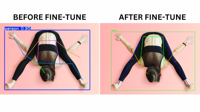
Evaluation, metrics, and validation strategy
Primary: mAP@0.5 and mAP@[0.5:0.95]. Report both.
Secondary: per-class AP, precision, recall, F1, confusion matrix.
Operational: latency, memory, inference throughput, and end-to-end pipeline time.
Hard negative analysis: sample top false positives and false negatives and triage their causes (label errors, domain gap, occlusion, small objects).
Ablations: test with/without pseudo labels, with varying
w_pseudo, and with/without synthetic data to measure marginal gains.
Ultralytics docs give practical evaluation insights and how to interpret mAP for detection tasks.
Experiment design and ablation checklist
For each experiment:
Fix random seed. Save seed and environment.
Save dataset commit id (dataset version hash).
Log model config, hyperparameters, augmentations, and number of pseudo labels.
Run at least 3 seeds for critical comparisons.
Compare on the human-verified validation set only.
Ablations to run:
prelabel vs no prelabel.
pseudo-label threshold sweep (e.g., 0.8, 0.9, 0.95).
pseudo weight sweep (e.g., 0.1, 0.3, 0.5).
synthetic fraction sweep (0%, 25%, 50%, 75% synthetic).
mosaic probability sweep.
CI/CD for models and datasets
Dataset CI: on dataset version push run quick QA checks (bbox inside image, missing files, class balance, distribution drift vs previous).
Training CI: run a smoke train on tiny subset and fail pipeline on obvious regressions.
Validation gate: require minimum mAP on validation and stable latency before automatic promotion.
Artifact storage: store
best.pt,last.pt, exported ONNX/TensorRT, and training logs. Tag by dataset and model commit.Canary: deploy to shadow environment and monitor errors for minimum time before full rollout.
Model export and edge optimizations
Export to ONNX then optimize to TensorRT for NVIDIA inference. For mobile, use TFLite or CoreML.
Quantization: FP16 first, then INT8 with calibration dataset if available. Validate on real data after quant.
Pruning: channel pruning for strict latency budgets. Retrain after pruning if needed.
Postprocessing: optimize NMS (fast NMS or Soft-NMS variants) and batched preprocessing.
Example Ultralytics export:
yolo export model=runs/detect/train/weights/best.pt format=onnx
Monitoring and drift detection
Monitor per-class confidence distributions and feature embeddings over time.
Periodically sample low-confidence predictions and push to an AL queue for human review.
Maintain a small rolling human-verified test set from production for continuous evaluation.
Trigger retrain when mAP drops by a configurable delta or when feature distribution divergence exceeds threshold.
Cost, human effort, and timeline estimates
Estimates are domain dependent. Ballpark for a medium domain (3–10 classes):
Seed labeling (1k labeled images): 1–3 weeks with a small team.
Prelabel + human correction (10k pool): 2–6 weeks with AL cycles.
Training runs and hyperparameter search: 1–3 weeks.
Production readiness: 4–12 weeks total.
Active learning and prelabeling commonly reduce labeling cost by 2–10× depending on domain maturity. Surveys and field studies confirm substantial gains when AL and prelabel are applied.
Common failure modes and fixes
Noisy pseudo labels degrade accuracy. Fix: raise teacher confidence threshold, add localization checks, lower
w_pseudo.Overfitting to synthetic styles. Fix: mix real data earlier, tune domain randomization, use style transfer as augmentation.
Small object recall collapse after resizing images too low. Fix: increase
imgsz, add small object augment, use FPN variants for higher feature resolution.Mosaic artifacts create impossible context. Fix: reduce mosaic probability or disable in final fine-tune.
Concrete active-learning + pseudo-label loop (pseudocode)
					# high-level pseudocode
for cycle in range(max_cycles):
    # 1. infer on unlabeled pool
    preds = model.predict(unlabeled_images, batch=bs)
    # 2. compute uncertainty and novelty
    scores = compute_score(preds, features, labeled_features)
    # 3. select top-K for annotation
    to_label = select_top_k(scores, K)
    annotated = annotator_api.label_images(to_label, prelabels=preds)
    # 4. add high-confidence preds as pseudo labels
    pseudo = [p for p in preds if p.confidence >= pseudo_thresh and loc_quality(p) >= loc_thresh]
    # 5. create training set with weights
    train_set = combine(human_labels, pseudo)  # with sample weights for pseudo
    # 6. train/fine-tune model
    model.train(train_set, epochs=E, lr=lr)
    # 7. evaluate on human-verified validation set
    val_metrics = model.eval(val_set)
    if val_metrics['mAP50_95'] improves < delta:
        break
Implement compute_score using ensemble disagreement or MC Dropout for stronger uncertainty.
Appendix A — Example data.yaml
					train: /mnt/data/dataset/train/images
val: /mnt/data/dataset/val/images
nc: 4
names: ['person','helmet','vest','tool']
Appendix B — Quick checklist before first production run
Seed dataset labeled and QA’d.
Validation set human-verified and isolated.
Spec versioned and published.
Baseline prelabel run done and annotator workflow tested.
AL selection script validated on a small pool.
Training configs and CLI tested in reproducible env.
Export and inference benchmark script validated.
Canary deployment plan created.
Conclusion
A production-grade YOLO fine-tuning program is an iterative systems problem, not a one-off training run. Start with a small, high-quality seed and automate the repetitive steps: prelabeling, selection, QA, and versioning. Use active learning and careful pseudo-label hygiene to scale while holding a strictly human-verified validation set as the single source of truth. Instrument every step with lineage, metrics, and CI gates so retraining becomes routine, auditable, and safe for deployment. Implement these elements and you convert manual labeling effort into a repeatable engine that delivers better detectors faster and with lower cost.


