
Introduction Computer vision has come a long way, but high-performing AI models often come with a catch: they’re huge, resource-hungry, and impractical for mobile devices. The original Segment Anything Model (SAM) broke ground in universal image segmentation, yet its massive size made real-time, on-device use nearly impossible. In this series, we explore Mobile Segment Anything (MobileSAM) — a lightweight, mobile-ready adaptation that brings powerful segmentation to smartphones, embedded systems, and edge devices. MobileSAM keeps the precision and flexibility of SAM while dramatically reducing computational demands, opening the door to real-time AI applications wherever you need them. From mobile photo editing to augmented reality, robotics, and even healthcare imaging, MobileSAM makes it possible to run sophisticated image segmentation directly on-device — fast, efficient, and without sacrificing privacy. In short, it’s AI vision, untethered. What Is MobileSAM? MobileSAM is a lightweight adaptation of the Segment Anything Model (SAM) designed to perform image segmentation with significantly reduced computational requirements. Image segmentation is the process of identifying and separating objects within an image at the pixel level. Instead of simply detecting objects, segmentation precisely outlines them. MobileSAM achieves this while maintaining strong accuracy but drastically improving speed and efficiency. Key Idea Replace heavy components of SAM with a compact encoder architecture while keeping the powerful segmentation capability intact. The result: Faster inference Lower memory usage Mobile compatibility Near-SAM performance Why MobileSAM Was Created The original SAM model introduced a universal segmentation approach capable of understanding almost any visual object. However, it required: High GPU power Large memory capacity Server-level hardware This limited real-world deployment. MobileSAM was developed to solve three major challenges: Edge deployment Real-time performance Energy efficiency Now segmentation can run directly on devices instead of relying on cloud processing. How MobileSAM Works MobileSAM keeps SAM’s general pipeline but optimizes the architecture. 1. Lightweight Image Encoder The main improvement lies in replacing SAM’s large Vision Transformer encoder with a smaller, mobile-friendly backbone. Benefits: Reduced parameters Faster computation Lower latency 2. Prompt-Based Segmentation Like SAM, MobileSAM accepts prompts such as: Points Bounding boxes Masks Text guidance (via integrations) Users can interactively guide segmentation results. 3. Efficient Mask Decoder The decoder remains similar to SAM, preserving segmentation quality while benefiting from the faster encoder. Key Features of MobileSAM Real-Time Performance MobileSAM runs significantly faster than traditional segmentation models, enabling live applications. Mobile & Edge Ready Designed for: Smartphones AR/VR devices Robotics systems IoT cameras General-Purpose Segmentation Works across diverse categories without retraining. Energy Efficient Lower computational demand means better battery performance. MobileSAM vs Original SAM Feature SAM MobileSAM Model Size Very Large Lightweight Hardware Needs GPU Required Mobile Compatible Speed Moderate Very Fast Edge Deployment Limited Excellent Accuracy Extremely High Near-Comparable MobileSAM trades a small amount of accuracy for massive gains in usability and speed. Real-World Use Cases 1. Mobile Photo Editing Apps Instant background removal and object selection directly on-device. 2. Augmented Reality (AR) Real-time object segmentation improves immersive AR experiences. 3. Robotics Robots can understand environments locally without cloud dependence. 4. Autonomous Systems Drones and smart vehicles benefit from lightweight perception models. 5. Healthcare Imaging Portable medical devices can analyze visuals offline. Advantages of On-Device Segmentation Running segmentation locally provides major benefits: Privacy protection (no cloud upload) Reduced latency Offline functionality Lower operational cost Improved responsiveness MobileSAM aligns perfectly with the growing trend of edge AI computing. Performance and Efficiency MobileSAM achieves: Dramatically reduced model size Faster inference speeds Comparable segmentation quality to SAM Lower power consumption This balance makes it practical for commercial applications where performance and efficiency must coexist. Developer Benefits Developers adopting MobileSAM gain: Easier deployment pipelines Reduced infrastructure costs Cross-platform compatibility Real-time interaction capabilities It integrates well with frameworks such as: PyTorch ONNX Mobile AI runtimes Challenges and Limitations Despite its advantages, MobileSAM still has trade-offs: Slight accuracy reduction compared to full SAM Performance varies across hardware Complex scenes may still require larger models However, ongoing optimization continues to close these gaps. The Future of Mobile Vision Models MobileSAM represents a broader shift toward efficient AI models rather than simply larger ones. Future trends include: Smaller multimodal models On-device generative AI Privacy-first AI applications Real-time AI assistants powered locally Lightweight models like MobileSAM are expected to become foundational for next-generation applications. Conclusion Mobile Segment Anything (MobileSAM) marks an important evolution in computer vision. By bringing powerful segmentation capabilities to mobile and edge devices, it removes one of the biggest barriers to deploying advanced AI in everyday environments. As AI moves from cloud servers to personal devices, MobileSAM demonstrates how efficiency, speed, and accessibility can coexist with high-quality performance. For developers, startups, and researchers, MobileSAM isn’t just an optimization — it’s a gateway to scalable, real-world AI vision systems. Visit Our Data Annotation Service Visit Now Lorem ipsum dolor sit amet, consectetur adipiscing elit. Ut elit tellus, luctus nec ullamcorper mattis, pulvinar dapibus leo.
Introduction Edge AI is transforming how computer vision systems are deployed, moving intelligence from the cloud directly onto devices operating in real time. NVIDIA Jetson platforms make this possible by combining GPU acceleration, low power consumption, and optimized AI software stacks. With the latest Ultralytics YOLO26 model, developers can achieve faster inference, improved detection accuracy, and efficient deployment on embedded systems. When combined with NVIDIA DeepStream SDK and TensorRT optimization, YOLO26 becomes a powerful solution for real-time video analytics at the edge. This guide walks through end-to-end integration of YOLO26 with DeepStream on Jetson, enabling scalable, production-ready object detection pipelines. Why DeepStream for Edge AI? Running raw inference scripts works for experimentation, but production deployments require: High-throughput video processing Hardware acceleration Multi-stream scalability Efficient memory handling Pipeline-based architecture DeepStream provides: ✅ GPU-accelerated video decoding✅ Zero-copy memory pipelines✅ Batch inference support✅ Built-in tracking and analytics✅ RTSP and camera streaming support Instead of processing frames manually, DeepStream builds optimized pipelines using GStreamer. System Architecture Overview The deployment stack looks like this: Camera / Video Stream ↓ Video Decode (NVDEC) ↓ DeepStream Pipeline ↓ TensorRT Engine (YOLO26) ↓ Object Detection Metadata ↓ Display / Stream / Analytics Key components: Component Purpose YOLO26 Object detection model TensorRT Optimized inference engine DeepStream Video analytics pipeline Jetson GPU Hardware acceleration Hardware Requirements Supported Jetson platforms: Jetson Nano (limited performance) Jetson Xavier NX Jetson AGX Xavier Jetson Orin Nano Jetson Orin NX Jetson AGX Orin (recommended) Recommended minimum: 8GB RAM JetPack 6.x CUDA + TensorRT installed Software Stack Ensure the following are installed: JetPack SDK CUDA Toolkit TensorRT DeepStream SDK Python 3.8+ Ultralytics framework Verify installation: deepstream-app –version-all Step 1 — Install Ultralytics YOLO26 Clone and install dependencies: pip install ultralytics Test inference: yolo predict model=yolo26.pt source=bus.jpg If inference works, proceed to export. Step 2 — Export YOLO26 to ONNX DeepStream uses TensorRT engines, so first export the model. yolo export model=yolo26.pt format=onnx opset=12 Output: yolo26.onnx Verify ONNX model: pip install onnxruntime python -c "import onnx; onnx.load('yolo26.onnx')" Step 3 — Convert ONNX to TensorRT Engine Use TensorRT to optimize inference for Jetson GPU. /usr/src/tensorrt/bin/trtexec –onnx=yolo26.onnx –saveEngine=yolo26.engine –fp16 Optional INT8 optimization (advanced): –int8 –calib=calibration.cache Benefits: Lower latency Reduced memory usage Hardware-specific optimization Step 4 — Integrate YOLO26 with DeepStream DeepStream requires a custom parser for YOLO outputs. Directory Structure deepstream_yolo26/ ├── config_infer_primary.txt ├── yolo26.engine ├── labels.txt └── custom_parser.cpp Configure Primary Inference Create: config_infer_primary.txt [property] gpu-id=0 net-scale-factor=0.003921569 model-engine-file=yolo26.engine labelfile-path=labels.txt batch-size=1 network-mode=2 num-detected-classes=80 process-mode=1 gie-unique-id=1 Network modes: 0 → FP32 1 → INT8 2 → FP16 Custom Bounding Box Parser YOLO models output tensors differently from standard detectors.You must implement a parser that converts raw outputs into: bounding boxes class IDs confidence scores Compile parser: make Output: LZ4ezwuSpTeD9pQKcUaPpHYUhy53QerXiD Step 5 — Modify DeepStream App Config Edit: deepstream_app_config.txt Set primary inference: [primary-gie] enable=1 config-file=config_infer_primary.txt Step 6 — Run DeepStream Pipeline Launch: deepstream-app -c deepstream_app_config.txt You should see: ✅ Real-time detections✅ Bounding boxes rendered✅ GPU utilization active Performance Optimization Tips 1. Use FP16 or INT8 FP16 typically provides: 2–3× faster inference Minimal accuracy loss INT8 gives maximum performance but requires calibration. 2. Increase Batch Size (Multi-Stream) batch-size=4 Useful for multiple RTSP cameras. 3. Enable Zero-Copy Memory DeepStream automatically uses NVMM buffers to avoid CPU copies. 4. Use Hardware Decoder Ensure pipeline uses: nvv4l2decoder instead of software decoding. Expected Performance (Approximate) Device FPS (YOLO26 FP16) Jetson Nano 6–10 FPS Xavier NX 25–40 FPS Orin Nano 40–70 FPS AGX Orin 90–150 FPS Performance varies with resolution and model size. Real-World Use Cases YOLO26 + DeepStream enables: Smart city surveillance Retail analytics Industrial safety monitoring Traffic analysis Robotics perception Autonomous inspection systems Troubleshooting Engine Not Loading Rebuild engine directly on Jetson: trtexec –onnx=model.onnx TensorRT engines are hardware-specific. No Bounding Boxes Appearing Check: parser library path class count output tensor names Low FPS Verify GPU usage: tegrastats Common causes: CPU decoding FP32 inference incorrect batch configuration Best Practices for Production Build TensorRT engines on target hardware Use RTSP streams for scalability Enable tracking plugins Log inference metadata Containerize with Docker Conclusion Integrating YOLO26 with DeepStream on NVIDIA Jetson unlocks a highly optimized edge AI pipeline capable of real-time video analytics at production scale. By combining: YOLO26 detection accuracy TensorRT acceleration DeepStream pipeline efficiency Jetson edge hardware developers can deploy scalable, low-latency AI systems without relying on cloud infrastructure. This workflow forms a strong foundation for next-generation edge vision applications across industries. Visit Our Data Annotation Service Visit Now
Introduction For nearly a decade, the YOLO (You Only Look Once) family has defined what real-time computer vision means. From the revolutionary YOLOv1 in 2015 to increasingly efficient and accurate successors, each generation has pushed the boundary between speed, accuracy, and deployability. In 2026, a new milestone arrived. YOLO26 is not just another incremental upgrade, it represents a fundamental redesign of how object detection systems are trained, optimized, and deployed, especially for edge devices and real-world AI systems. Built with an edge-first philosophy, YOLO26 introduces end-to-end detection without traditional post-processing, improved stability during training, and multi-task vision capabilities, making it one of the most practical computer vision models ever released. This article explores: ✅ The evolution leading to YOLO26✅ Architecture innovations✅ Why NMS-free detection matters✅ Performance improvements✅ Real-world applications✅ How developers can use YOLO26 today✅ The future of vision AI The Journey to YOLO26 Object detection historically struggled with a difficult trade-off: Faster models sacrificed accuracy Accurate models required heavy computation Real-time deployment remained difficult Earlier YOLO versions gradually solved these problems: YOLOv5–v8 improved usability and modular training YOLOv9–v11 introduced smarter gradient learning and efficiency improvements YOLOv10 began moving toward end-to-end detection pipelines YOLO26 completes this transition. Instead of patching limitations with additional heuristics, it redesigns the pipeline itself. Research analyzing the model highlights that YOLO26 establishes a new efficiency–accuracy balance while outperforming many previous detectors in both speed and precision. What Is YOLO26? YOLO26 is a real-time, multi-task computer vision model optimized for: Object detection Instance segmentation Pose estimation Tracking Classification Unlike earlier detectors, YOLO26 is designed primarily for edge deployment, meaning it runs efficiently on: CPUs Mobile devices Embedded systems Robotics hardware Jetson and ARM platforms The model supports scalable sizes, allowing developers to choose between lightweight and high-accuracy configurations depending on hardware constraints. The Biggest Breakthrough: NMS-Free Detection The Problem with Traditional YOLO Previous YOLO models relied on Non-Maximum Suppression (NMS). NMS removes duplicate bounding boxes after prediction — but it introduces problems: Extra latency Hyperparameter tuning complexity Instability in crowded scenes Deployment inconsistencies YOLO26 Solution YOLO26 eliminates NMS entirely. Instead, detection becomes fully end-to-end — predictions are learned directly during training rather than filtered afterward. This change: Reduces inference time Simplifies deployment Improves consistency across devices Researchers note that removing heuristic post-processing resolves long-standing latency vs. precision trade-offs in object detection systems. Key Architectural Innovations YOLO26 introduces several new mechanisms. 1. Progressive Loss Balancing (ProgLoss) Training object detectors often suffers from unstable gradients. ProgLoss dynamically adjusts learning emphasis during training, allowing: Faster convergence Improved generalization Stable optimization on small datasets 2. Small-Target-Aware Label Assignment (STAL) Small objects are traditionally difficult to detect. STAL improves label assignment by prioritizing tiny and distant objects — critical for: Surveillance Drone imagery Autonomous driving Medical imaging 3. MuSGD Optimizer Inspired by optimization strategies used in large AI models, MuSGD improves: Training stability Quantization readiness Low-precision deployment 4. Removal of Distribution Focal Loss (DFL) Earlier YOLO versions used complex bounding box regression losses. YOLO26 simplifies this pipeline, enabling: Easier export to ONNX/TensorRT Faster inference Reduced memory overhead Where YOLOv1 Fell Short, and Why That’s Important YOLOv1’s limitations weren’t accidental; they revealed deep insights. Small Objects Grid resolution limited detection granularity Small objects often disappeared within grid cells Crowded Scenes One object class prediction per cell Overlapping objects confused the model Localization Precision Coarse bounding box predictions Lower IoU scores than region-based methods Each weakness became a research question that drove YOLOv2, YOLOv3, and beyond. Edge-First Design Philosophy One of YOLO26’s defining goals is predictable latency. Traditional models were GPU-centric. YOLO26 focuses on: CPU acceleration Embedded inference Low-power AI devices Benchmarks show significant CPU inference improvements and reliable performance even without GPUs. This shift makes AI accessible beyond data centers. Performance Improvements YOLO26 improves across three critical axes: Speed Faster inference due to NMS removal Reduced computational overhead Accuracy Better small-object detection Improved dense-scene performance Efficiency Smaller models with higher mAP Stable quantization for edge deployment Studies comparing YOLO26 with earlier generations highlight superior deployment versatility and efficiency across edge hardware platforms. Multi-Task Vision: One Model, Many Tasks YOLO26 moves toward unified vision AI. Supported tasks include: Detection Segmentation Pose estimation Tracking Oriented bounding boxes This reduces the need to maintain separate models for each task, simplifying production pipelines. Real-World Applications YOLO26 unlocks new possibilities across industries. Autonomous Systems Robots navigating dynamic environments Drone inspection systems Smart Cities Traffic monitoring Crowd analysis Security automation Healthcare Real-time medical imaging assistance Surgical instrument tracking Manufacturing Defect detection Quality assurance automation Retail & Logistics Shelf analytics Warehouse automation Because it runs efficiently on edge devices, processing can happen locally — improving privacy and reducing cloud costs. Developer Experience One reason YOLO became dominant is usability — and YOLO26 continues that tradition. Developers benefit from: Simple training pipelines Export to multiple runtimes Easy fine-tuning Real-time video inference Typical workflow: Prepare dataset Train using pretrained weights Export model Deploy on edge device No complex post-processing configuration required. YOLO26 vs Previous YOLO Versions Feature YOLOv8–11 YOLO26 NMS Required Yes No Edge Optimization Moderate Native Multi-Task Support Partial Unified Training Stability Good Improved Deployment Complexity Medium Low YOLO26 marks the transition from fast detectors to deployment-ready AI systems. Challenges and Limitations Despite improvements, challenges remain: Dense overlapping scenes still difficult Training large datasets remains compute-heavy Open-vocabulary detection is limited Transformer integration still evolving Future models may combine YOLO efficiency with foundation-model reasoning. The Future After YOLO26 YOLO26 signals a broader shift in computer vision: 👉 From GPU-centric AI → Edge AI👉 From pipelines → End-to-end learning👉 From single-task → unified perception systems Future developments may include: Vision-language integration Self-supervised detection On-device continual learning Autonomous AI perception stacks Conclusion YOLO26 is more than a version update. It represents a philosophical shift in computer vision engineering — simplifying architecture while improving real-world performance. By removing legacy bottlenecks like NMS, introducing smarter training strategies, and prioritizing edge deployment, YOLO26 brings AI closer to where it matters most: the real world. As AI moves beyond research labs into everyday devices, models like
Introduction Before YOLO, computers didn’t see the world the way humans do. They inspected it slowly, cautiously, one object proposal at a time. Object detection worked, but it was fragmented, computationally expensive, and far from real time. Then, in 2015, a single paper changed everything. “You Only Look Once: Unified, Real-Time Object Detection” by Joseph Redmon et al. introduced YOLOv1, a model that redefined how machines perceive images. It wasn’t just an incremental improvement, it was a conceptual revolution. This is the story of how YOLOv1 was born, how it worked, and why its impact still echoes across modern computer vision systems today. Object Detection Before YOLO: A Fragmented World Before YOLOv1, object detection research was dominated by complex pipelines stitched together from multiple independent components. Each component worked reasonably well on its own, but the overall system was fragile, slow, and difficult to optimize. The Classical Detection Pipeline A typical object detection system before 2015 looked like this: Hand-crafted or heuristic-based region proposal Selective Search Edge Boxes Sliding windows (earlier methods) Feature extraction CNN features (AlexNet, VGG, etc.) Run separately on each proposed region Classification SVMs or softmax classifiers One classifier per region Bounding box regression Fine-tuning box coordinates post-classification Each stage was trained independently, often with different objectives. Why This Was a Problem Redundant computationThe same image features were recomputed hundreds of times. No global contextThe model never truly “saw” the full image at once. Pipeline fragilityErrors in region proposals could never be recovered downstream. Poor real-time performanceEven Fast R-CNN struggled to exceed a few FPS. Object detection worked, but it felt like a workaround, not a clean solution. The YOLO Philosophy: Detection as a Single Learning Problem YOLOv1 challenged the dominant assumption that object detection must be a multi-stage problem. Instead, it asked a radical question: Why not predict everything at once, directly from pixels? A Conceptual Shift YOLO reframed object detection as: A single regression problem from image pixels to bounding boxes and class probabilities. This meant: No region proposals No sliding windows No separate classifiers No post-hoc stitching Just one neural network, trained end-to-end. Why This Matters This shift: Simplified the learning objective Reduced engineering complexity Allowed gradients to flow across the entire detection task Enabled true real-time inference YOLO didn’t just optimize detection, it redefined what detection was. How YOLOv1 Works: A New Visual Grammar YOLOv1 introduced a structured way for neural networks to “describe” an image. Grid-Based Responsibility Assignment The image is divided into an S × S grid (commonly 7 × 7). Each grid cell: Is responsible for objects whose center lies within it Predicts bounding boxes and class probabilities This created a spatial prior that helped the network reason about where objects tend to appear. Bounding Box Prediction Details Each grid cell predicts B bounding boxes, where each box consists of: x, y → center coordinates (relative to the grid cell) w, h → width and height (relative to the image) confidence score The confidence score encodes: Pr(object) × IoU(predicted box, ground truth) This was clever, it forced the network to jointly reason about objectness and localization quality. Class Prediction Strategy Instead of predicting classes per bounding box, YOLOv1 predicted: One set of class probabilities per grid cell This reduced complexity but introduced limitations in crowded scenes, a trade-off YOLOv1 knowingly accepted. YOLOv1 Architecture: Designed for Global Reasoning YOLOv1’s network architecture was intentionally designed to capture global image context. Architecture Breakdown 24 convolutional layers 2 fully connected layers Inspired by GoogLeNet (but simpler) Pretrained on ImageNet classification The final fully connected layers allowed YOLO to: Combine spatially distant features Understand object relationships Avoid false positives caused by local texture patterns Why Global Context Matters Traditional detectors often mistook: Shadows for objects Textures for meaningful regions YOLO’s global reasoning reduced these errors by understanding the scene as a whole. The YOLOv1 Loss Function: Balancing Competing Objectives Training YOLOv1 required solving a delicate optimization problem. Multi-Part Loss Components YOLOv1’s loss function combined: Localization loss Errors in x, y, w, h Heavily weighted to prioritize accurate boxes Confidence loss Penalized incorrect objectness predictions Classification loss Penalized wrong class predictions Smart Design Choices Higher weight for bounding box regression Lower weight for background confidence Square root applied to width and height to stabilize gradients These design choices directly influenced how future detection losses were built. Speed vs Accuracy: A Conscious Design Trade-Off YOLOv1 was explicit about its priorities. YOLO’s Position Slightly worse localization is acceptable if it enables real-time vision. Performance Impact YOLOv1 ran an order of magnitude faster than competing detectors Enabled deployment on: Live camera feeds Robotics systems Embedded devices (with Fast YOLO) This trade-off reshaped how researchers evaluated detection systems, not just by accuracy, but by usability. Where YOLOv1 Fell Short, and Why That’s Important YOLOv1’s limitations weren’t accidental; they revealed deep insights. Small Objects Grid resolution limited detection granularity Small objects often disappeared within grid cells Crowded Scenes One object class prediction per cell Overlapping objects confused the model Localization Precision Coarse bounding box predictions Lower IoU scores than region-based methods Each weakness became a research question that drove YOLOv2, YOLOv3, and beyond. Why YOLOv1 Changed Computer Vision Forever YOLOv1 didn’t just introduce a model, it introduced a mindset. End-to-End Learning as a Principle Detection systems became: Unified Differentiable Easier to deploy and optimize Real-Time as a First-Class Metric After YOLO: Speed was no longer optional Real-time inference became an expectation A Blueprint for Future Detectors Modern architectures, CNN-based and transformer-based alike, inherit YOLO’s core ideas: Dense prediction Single-pass inference Deployment-aware design Final Reflection: The Day Detection Became Vision YOLOv1 marked the moment when object detection stopped being a patchwork of tricks and became a coherent vision system. It taught the field that: Seeing fast unlocks new realities Simplicity scales End-to-end learning changes how machines understand the world YOLO didn’t just look once. It made computer vision see differently forever. Visit Our Data Annotation Service Visit Now Lorem ipsum dolor sit amet, consectetur adipiscing elit. Ut elit tellus, luctus nec
Introduction Artificial intelligence has been circling healthcare for years, diagnosing images, summarizing clinical notes, predicting risks, yet much of its real power has remained locked behind proprietary walls. Google’s MedGemma changes that equation. By releasing open medical AI models built specifically for healthcare contexts, Google is signaling a shift from “AI as a black box” to AI as shared infrastructure for medicine. This is not just another model release. MedGemma represents a structural change in how healthcare AI can be developed, validated, and deployed. The Problem With Healthcare AI So Far Healthcare AI has faced three persistent challenges: OpacityMany high-performing medical models are closed. Clinicians cannot inspect them, regulators cannot fully audit them, and researchers cannot adapt them. General Models, Specialized RisksLarge general-purpose language models are not designed for clinical nuance. Small mistakes in medicine are not “edge cases”, they are liability. Inequitable AccessAdvanced medical AI often ends up concentrated in large hospitals, well-funded startups, or high-income countries. The result is a paradox: AI shows promise in healthcare, but trust, scalability, and equity remain unresolved. What Is MedGemma? MedGemma is a family of open-weight medical AI models released by Google, built on the Gemma architecture but adapted specifically for healthcare and biomedical use cases. Key characteristics include: Medical-domain tuning (clinical language, biomedical concepts) Open weights, enabling inspection, fine-tuning, and on-prem deployment Designed for responsible use, with explicit positioning as decision support, not clinical authority In simple terms: MedGemma is not trying to replace doctors. It is trying to become a reliable, transparent assistant that developers and institutions can actually trust. Why “Open” Matters More in Medicine Than Anywhere Else In most consumer applications, closed models are an inconvenience. In healthcare, they are a risk. Transparency and Auditability Open models allow: Independent evaluation of bias and failure modes Regulatory scrutiny Reproducible research This aligns far better with medical ethics than “trust us, it works.” Customization for Real Clinical Settings Hospitals differ. So do patient populations. Open models can be fine-tuned for: Local languages Regional disease prevalence Institutional workflows Closed APIs cannot realistically offer this depth of adaptation. Data Privacy and Sovereignty With MedGemma, organizations can: Run models on-premises Keep patient data inside institutional boundaries Comply with strict data protection regulations For healthcare systems, this is not optional, it is mandatory. Potential Use Cases That Actually Make Sense MedGemma is not a silver bullet, but it enables realistic, high-impact applications: 1. Clinical Documentation Support Drafting summaries from structured notes Translating between clinical and patient-friendly language Reducing physician burnout (quietly, which is how doctors prefer it) 2. Medical Education and Training Interactive case simulations Question-answering grounded in medical terminology Localized medical training tools in under-resourced regions 3. Research Acceleration Literature review assistance Hypothesis exploration Data annotation support for medical datasets 4. Decision Support (Not Decision Making) Flagging potential issues Surfacing relevant guidelines Assisting, not replacing, clinical judgment The distinction matters. MedGemma is positioned as a copilot, not an autopilot. Safety, Responsibility, and the Limits of AI Google has been explicit about one thing: MedGemma is not a diagnostic authority. This is important for two reasons: Legal and Ethical RealityMedicine requires accountability. AI cannot be held accountable, people can. Trust Through ConstraintModels that openly acknowledge their limits are more trustworthy than those that pretend omniscience. MedGemma’s real value lies in supporting human expertise, not competing with it. How MedGemma Could Shift the Healthcare AI Landscape From Products to Platforms Instead of buying opaque AI tools, hospitals can build their own systems on top of open foundations. From Vendor Lock-In to Ecosystems Researchers, startups, and institutions can collaborate on improvements rather than duplicating effort behind closed doors. From “AI Hype” to Clinical Reality Open evaluation encourages realistic benchmarking, failure analysis, and incremental improvement, exactly how medicine advances. The Bigger Picture: Democratizing Medical AI Healthcare inequality is not just about access to doctors, it is about access to knowledge. Open medical AI models: Lower barriers for low-resource regions Enable local innovation Reduce dependence on external vendors If used responsibly, MedGemma could help ensure that medical AI benefits are not limited to the few who can afford them. Final Thoughts Google’s MedGemma is not revolutionary because it is powerful. It is revolutionary because it is open, medical-first, and constrained by responsibility. In a field where trust matters more than raw capability, that may be exactly what healthcare AI needs. The real transformation will not come from AI replacing clinicians, but from clinicians finally having AI they can understand, adapt, and trust. Visit Our Data Annotation Service Visit Now Lorem ipsum dolor sit amet, consectetur adipiscing elit. Ut elit tellus, luctus nec ullamcorper mattis, pulvinar dapibus leo.
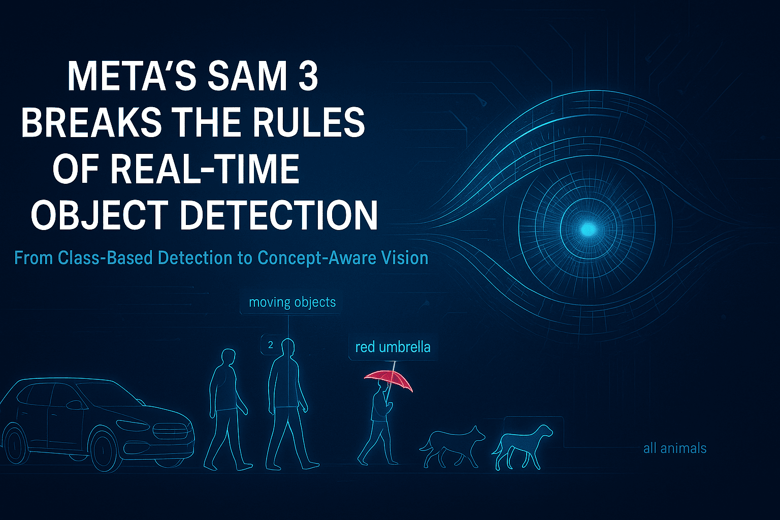
Introduction For years, real-time object detection has followed the same rigid blueprint: define a closed set of classes, collect massive labeled datasets, train a detector, bolt on a segmenter, then attach a tracker for video. This pipeline worked—but it was fragile, expensive, and fundamentally limited. Any change in environment, object type, or task often meant starting over. Meta’s Segment Anything Model 3 (SAM 3) breaks this cycle entirely. As described in the Coding Nexus analysis, SAM 3 is not just an improvement in accuracy or speed—it is a structural rethinking of how object detection, segmentation, and tracking should work in modern computer vision systems . SAM 3 replaces class-based detection with concept-based understanding, enabling real-time segmentation and tracking using simple natural-language prompts. This shift has deep implications across robotics, AR/VR, video analytics, dataset creation, and interactive AI systems. 1. The Core Problem With Traditional Object Detection Before understanding why SAM 3 matters, it’s important to understand what was broken. 1.1 Rigid Class Definitions Classic detectors (YOLO, Faster R-CNN, SSD) operate on a fixed label set. If an object category is missing—or even slightly redefined—the model fails. “Dog” might work, but “small wet dog lying on the floor” does not. 1.2 Fragmented Pipelines A typical real-time vision system involves: A detector for bounding boxes A segmenter for pixel masks A tracker for temporal consistency Each component has its own failure modes, configuration overhead, and performance tradeoffs. 1.3 Data Dependency Every new task requires new annotations. Collecting and labeling data often costs more than training the model itself. SAM 3 directly targets all three issues. 2. SAM 3’s Conceptual Breakthrough: From Classes to Concepts The most important innovation in SAM 3 is the move from class-based detection to concept-based segmentation. Instead of asking: “Is there a car in this image?” SAM 3 answers: “Show me everything that matches this concept.” That concept can be expressed as: a short text phrase a descriptive noun group or a visual example This approach is called Promptable Concept Segmentation (PCS) . Why This Matters Concepts are open-ended No retraining is required The same model works across images and videos Semantic understanding replaces rigid taxonomy This fundamentally changes how humans interact with vision systems. 3. Unified Detection, Segmentation, and Tracking SAM 3 eliminates the traditional multi-stage pipeline. What SAM 3 Does in One Pass Detects all instances of a concept Produces pixel-accurate masks Assigns persistent identities across video frames Unlike earlier SAM versions, which segmented one object per prompt, SAM 3 returns all matching instances simultaneously, each with its own identity for tracking . This makes real-time video understanding far more robust, especially in crowded or dynamic scenes. 4. How SAM 3 Works (High-Level Architecture) While the Medium article avoids low-level math, it highlights several key architectural ideas: 4.1 Language–Vision Alignment Text prompts are embedded into the same representational space as visual features, allowing semantic matching between words and pixels. 4.2 Presence-Aware Detection SAM 3 doesn’t just segment—it first determines whether a concept exists in the scene, reducing false positives and improving precision. 4.3 Temporal Memory For video, SAM 3 maintains internal memory so objects remain consistent even when: partially occluded temporarily out of frame changing shape or scale This is why SAM 3 can replace standalone trackers. 5. Real-Time Performance Implications A key insight from the article is that real-time no longer means simplified models. SAM 3 demonstrates that: High-quality segmentation Open-vocabulary understanding Multi-object tracking can coexist in a single real-time system—provided the architecture is unified rather than modular . This redefines expectations for what “real-time” vision systems can deliver. 6. Impact on Dataset Creation and Annotation One of the most immediate consequences of SAM 3 is its effect on data pipelines. Traditional Annotation Manual labeling Long turnaround times High cost per image or frame With SAM 3 Prompt-based segmentation generates masks instantly Humans shift from labeling to verification Dataset creation scales dramatically faster This is especially relevant for industries like autonomous driving, medical imaging, and robotics, where labeled data is a bottleneck. 7. New Possibilities in Video and Interactive Media SAM 3 enables entirely new interaction patterns: Text-driven video editing Semantic search inside video streams Live AR effects based on descriptions, not predefined objects For example: “Highlight all moving objects except people.” Such instructions were impractical with classical detectors but become natural with SAM 3’s concept-based approach. 8. Comparison With Previous SAM Versions Feature SAM / SAM 2 SAM 3 Object count per prompt One All matching instances Video tracking Limited / external Native Vocabulary Implicit Open-ended Pipeline complexity Moderate Unified Real-time use Experimental Practical SAM 3 is not a refinement—it is a generational shift. 9. Current Limitations Despite its power, SAM 3 is not a silver bullet: Compute requirements are still significant Complex reasoning (multi-step instructions) requires external agents Edge deployment remains challenging without distillation However, these are engineering constraints, not conceptual ones. 10. Why SAM 3 Represents a Structural Shift in Computer Vision SAM 3 changes the role of object detection in AI systems: From rigid perception → flexible understanding From labels → language From pipelines → unified models As emphasized in the Coding Nexus article, this shift is comparable to the jump from keyword search to semantic search in NLP . Final Thoughts Meta’s SAM 3 doesn’t just improve object detection—it redefines how humans specify visual intent. By making language the interface and concepts the unit of understanding, SAM 3 pushes computer vision closer to how people naturally perceive the world. In the long run, SAM 3 is less about segmentation masks and more about a future where vision systems understand what we mean, not just what we label. Visit Our Data Annotation Service Visit Now
Introduction In computer vision, segmentation used to feel like the “manual labor” of AI: click here, draw a box there, correct that mask, repeat a few thousand times, try not to cry. Meta’s original Segment Anything Model (SAM) turned that grind into a point-and-click magic trick: tap a few pixels, get a clean object mask. SAM 2 pushed further to videos, bringing real-time promptable segmentation to moving scenes. Now SAM 3 arrives as the next major step: not just segmenting things you click, but segmenting concepts you describe. Instead of manually hinting at each object, you can say “all yellow taxis” or “players wearing red jerseys” and let the model find, segment, and track every matching instance in images and videos. This blog goes inside SAM 3—what it is, how it differs from its predecessors, what “Promptable Concept Segmentation” really means, and how it changes the way we think about visual foundation models. 1. From SAM to SAM 3: A short timeline Before diving into SAM 3, it helps to step back and see how we got here. SAM (v1): Click-to-segment The original SAM introduced a powerful idea: a large, generalist segmentation model that could segment “anything” given visual prompts—points, boxes, or rough masks. It was trained on a massive, diverse dataset and showed strong zero-shot segmentation performance across many domains. SAM 2: Images and videos, in real time SAM 2 extended the concept to video, treating an image as just a one-frame video and adding a streaming memory mechanism to support real-time segmentation over long sequences. Key improvements in SAM 2: Unified model for images and videos Streaming memory for efficient video processing Model-in-the-loop data engine to build a huge SA-V video segmentation dataset But SAM 2 still followed the same interaction pattern: you specify a particular location (point/box/mask) and get one object instance back at a time. SAM 3: From “this object” to “this concept” SAM 3 changes the game by introducing Promptable Concept Segmentation (PCS)—instead of saying “segment the thing under this click,” you can say “segment every dog in this video” and get: All instances of that concept Segmentation masks for each instance Consistent identities for each instance across frames (tracking) In other words, SAM 3 is no longer just a segmentation tool—it’s a unified, open-vocabulary detection, segmentation, and tracking model for images and videos. 2. What exactly is SAM 3? At its core, SAM 3 is a unified foundation model for promptable segmentation in images and videos that operates on concept prompts. Core capabilities According to Meta’s release and technical overview, SAM 3 can: Detect and segment objects Given a text or visual prompt, SAM 3 finds all matching object instances in an image or video and returns instance masks. Track objects over time For video, SAM 3 maintains stable identities, so the same object can be followed across frames. Work with multiple prompt types Text: “yellow school bus”, “person wearing a backpack” Image exemplars: example boxes/masks of an object Visual prompts: points, boxes, masks (SAM 2-style) Combined prompts: e.g., “red car” + one exemplar, for even sharper control Support open-vocabulary segmentation It doesn’t rely on a closed set of pre-defined classes. Instead, it uses language prompts and exemplars to generalize to new concepts. Scale to large image/video collections SAM 3 is explicitly designed to handle the “find everything like X” problem across large datasets, not just a single frame. Compared to SAM 2, SAM 3 formalizes PCS and adds language-driven concept understanding while preserving (and improving) the interactive segmentation capabilities of earlier versions. 3. Promptable Concept Segmentation (PCS): The big idea “Promptable Concept Segmentation” is the central new task that SAM 3 tackles. You provide a concept prompt, and the model returns masks + IDs for all objects matching that concept. Concept prompts can be: Text prompts Simple noun phrases like “red apple”, “striped cat”, “football player in blue”, “car in the left lane”. Image exemplars Positive/negative example boxes around objects you care about. Combined prompts Text + exemplars, e.g., “delivery truck” plus one example bounding box to steer the model. This is fundamentally different from classic SAM-style visual prompts: Feature SAM / SAM 2 SAM 3 (PCS) Prompt type Visual (points/boxes/masks) Text, exemplars, visual, or combinations Output per prompt One instance per interaction All instances of the concept Task scope Local, instance-level Global, concept-level across frame(s) Vocabulary Implicit, not language-driven Open-vocabulary via text + exemplars This means you can do things like: “Find every motorcycle in this 10-minute traffic video.” “Segment all people wearing helmets in a construction site dataset.” “Count all green apples versus red apples in a warehouse scan.” All without manually clicking each object. The dream of “query-like segmentation at scale” is much closer to reality. 4. Under the hood: How SAM 3 works (conceptually) Meta has published an overview and open-sourced the reference implementation via GitHub and model hubs such as Hugging Face. While the exact implementation details are in the official paper and code, the high-level ingredients look roughly like this: Vision backbone A powerful image/video encoder transforms each frame into a rich spatiotemporal feature representation. Concept encoder (language + exemplars) Text prompts are encoded using a language model or text encoder. Visual exemplars (e.g., boxes/masks around an example object) are encoded as visual features. The system fuses these into a concept embedding that represents “what you’re asking for”. Prompt–vision fusion The concept embedding interacts with the visual features (e.g., via attention) to highlight regions that correspond to the requested concept. Instance segmentation head From the fused feature map, the model produces: Binary/soft masks Instance IDs Optional detection boxes or scores Temporal component for tracking For video, SAM 3 uses mechanisms inspired by SAM 2’s streaming memory to maintain consistent identities for objects across frames, enabling efficient concept tracking over time. You can think of SAM 3 as “SAM 2 + a powerful vision-language concept engine,” wrapped into a single unified model. 5. SAM 3 vs SAM 2 and traditional detectors How does SAM 3 actually compare
Introduction Fine-tuning a YOLO model is a targeted effort to adapt powerful, pretrained detectors to a specific domain. The hard part is not the network. It is getting the right labelled data, at scale, with repeatable quality. An automated data-labeling pipeline combines model-assisted prelabels, active learning, pseudo-labeling, synthetic data and human verification to deliver that data quickly and cheaply. This guide shows why that pipeline matters, how its stages fit together, and which controls and metrics keep the loop reliable so you can move from a small seed dataset to a production-ready detector with predictable cost and measurable gains. Target audience and assumptions This guide assumes: You use YOLO (v8+ or similar Ultralytics family). You have access to modest GPU resources (1–8 GPUs). You can run a labeling UI with prelabel ingestion (CVAT, Label Studio, Roboflow, Supervisely). You aim for production deployment on cloud or edge. End-to-end pipeline (high level) Data ingestion: cameras, mobile, recorded video, public datasets, client uploads. Preprocess: frame extraction, deduplication, scene grouping, metadata capture. Prelabel: run a baseline detector to create model suggestions. Human-in-the-loop: annotators correct predictions. Active learning: select most informative images for human review. Pseudo-labeling: teacher model labels high-confidence unlabeled images. Combine, curate, augment, and convert to YOLO/COCO. Fine-tune model. Track experiments. Export, optimize, deploy. Monitor and retrain. Design each stage for automation via API hooks and version control for datasets and specs. Data collection and organization Inputs and signals to collect for every file: source id, timestamp, camera metadata, scene id, originating video id, uploader id. label metadata: annotator id, review pass, annotation confidence, label source (human/pseudo/prelabel/synthetic).Store provenance. Use scene/video grouping to create train/val splits that avoid leakage. Target datasets: Seed: 500–2,000 diverse images with human labels (task dependant). Scaling pool: 10k–100k+ unlabeled frames for pseudo/AL. Validation: 500–2,000 strictly human-verified images. Never mix pseudo labels into validation. Label ontology and specification Keep class set minimal and precise. Avoid overlapping classes. Produce a short spec: inclusion rules, occlusion thresholds, truncated objects, small object policy. Include 10–20 exemplar images per rule. Version the spec and require sign-off before mass labeling. Track label lineage in a lightweight DB or metadata store. Pre-labeling (model-assisted) Why: speeds annotators by 2–10x. How: Run a baseline YOLO (pretrained) across unlabeled pool. Save predictions in standard format (.txt or COCO JSON). Import predictions as an annotation layer in UI. Mark bounding boxes with prediction confidence. Present annotators only images above a minimum score threshold or with predicted classes absent in dataset to increase yield. Practical command (Ultralytics): yolo detect predict model=yolov8n.pt source=/data/pool imgsz=640 conf=0.15 save=True Adjust conf to control annotation effort. See Ultralytics fine-tuning docs for details. Human-in-the-loop workflow and QA Workflow: Pull top-K pre-labeled images into annotation UI. Present predicted boxes editable by annotator. Show model confidence. Enforce QA review on a stratified sample. Require second reviewer on disagreement. Flag images with ambiguous cases for specialist review. Quality controls: Inter-annotator agreement tracking. Random audit sampling. Automatic bounding-box sanity checks.Log QA metrics and use them in dataset weighting. Active learning: selection strategies Active learning reduces labeling needs by focusing human effort. Use a hybrid selection score: Selection score = α·uncertainty + β·novelty + γ·diversity Where: uncertainty = 1 − max_class_confidence across detections. novelty = distance in feature space from labeled set (use backbone features). diversity = clustering score to avoid redundant images. Common acquisition functions: Uncertainty sampling (low confidence). Margin sampling (difference between top two class scores). Core-set selection (max coverage). Density-weighted uncertainty (prioritize uncertain images in dense regions). Recent surveys on active learning show systematic gains and strong sample efficiency improvements. Use ensembles or MC-Dropout for improved uncertainty estimates. Pseudo-labeling and semi-supervised expansion Pseudo-labeling lets you expand labeled data cheaply. Risks: noisy boxes hurt learning. Controls: Teacher strength: prefer a high-quality teacher model (larger backbone or ensemble). Dual thresholds: classification_confidence ≥ T_cls (e.g., 0.9). localization_quality ≥ T_loc (e.g., IoU proxy or center-variance metric). Weighting: add pseudo samples with lower loss weight w_pseudo (e.g., 0.1–0.5) or use sample reweighting by teacher confidence. Filtering: apply density-guided or score-consistency filters to remove dense false positives. Consistency training: augment pseudo examples and enforce stable predictions (consistency loss). Seminal methods like PseCo and followups detail localization-aware pseudo labels and consistency training. These approaches improve pseudo-label reliability and downstream performance. Synthetic data and domain randomization When real data is rare or dangerous to collect, generate synthetic images. Best practices: Use domain randomization: vary lighting, textures, backgrounds, camera pose, noise, and occlusion. Mix synthetic and real: pretrain on synthetic, then fine-tune on small real set. Validate on held-out real validation set. Synthetic validation metrics often overestimate real performance; always check on real data. Recent studies in manufacturing and robotics confirm these tradeoffs. Tools: Blender+Python, Unity Perception, NVIDIA Omniverse Replicator. Save segmentation/mask/instance metadata for downstream tasks. Augmentation policy (practical) YOLO benefits from on-the-fly strong augmentation early in training, and reduced augmentation in final passes. Suggested phased policy: Phase 1 (warmup, epochs 0–20): aggressive augment. Mosaic, MixUp, random scale, color jitter, blur, JPEG corruption. Phase 2 (mid training, epochs 21–60): moderate augment. Keep Mosaic but lower probability. Phase 3 (final fine-tune, last 10–20% epochs): minimal augment to let model settle. Notes: Mosaic helps small object learning but may introduce unnatural context. Reduce mosaic probability in final phases. Use CutMix or copy-paste to balance rare classes. Do not augment validation or test splits. Ultralytics docs include augmentation specifics and recommended settings. YOLO fine-tuning recipes (detailed) Choose starting model based on latency/accuracy tradeoff: Iteration / prototyping: yolov8n (nano) or yolov8s (small). Production: yolov8m or yolov8l/x depending on target. Standard recipe: Prepare data.yaml: train: /data/train/images val: /data/val/images nc: names: [‘class0′,’class1’,…] 2. Stage 1 — head only: yolo detect train model=yolov8n.pt data=data.yaml epochs=25 imgsz=640 batch=32 freeze=10 lr0=0.001 3. Stage 2 — unfreeze full model: yolo detect train model=runs/train/weights/last.pt data=data.yaml epochs=75 imgsz=640 batch=16 lr0=0.0003 4. Final sweep: lower LR, turn off heavy augmentations, train few epochs to stabilize. Hyperparameter notes: Optimizer: SGD with momentum 0.9 usually generalizes better for detection. AdamW works for quick convergence. LR: warmup, cosine decay recommended. Start LR based
Introduction In 2025, choosing the right large language model (LLM) is about value, not hype. The true measure of performance is how well a model balances cost, accuracy, and latency under real workloads. Every token costs money, every delay affects user experience, and every wrong answer adds hidden rework. The market now centers on three leaders: OpenAI, Google, and Anthropic. OpenAI’s GPT-4o mini focuses on balanced efficiency, Google’s Gemini 2.5 lineup scales from high-end Pro to budget Flash tiers, and Anthropic’s Claude Sonnet 4.5 delivers top reasoning accuracy at a premium. This guide compares them side by side to show which model delivers the best performance per dollar for your specific use case. Pricing Snapshot (Representative) Provider Model / Tier Input ($/MTok) Output ($/MTok) Notes OpenAI GPT-4o mini $0.60 $2.40 Cached inputs available; balanced for chat and RAG. Anthropic Claude Sonnet 4.5 $3 $15 High output cost; excels on hard reasoning and long runs. Google Gemini 2.5 Pro $1.25 $10 Strong multimodal performance; tiered above 200k tokens. Google Gemini 2.5 Flash $0.30 $2.50 Low-latency, high-throughput. Batch discounts possible. Google Gemini 2.5 Flash-Lite $0.10 $0.40 Lowest-cost option for bulk transforms and tagging. Accuracy: Choose by Failure Cost Public leaderboards shift rapidly. Typical pattern: – Claude Sonnet 4.5 often wins on complex or long-horizon reasoning. Expect fewer ‘almost right’ answers.– Gemini 2.5 Pro is strong as a multimodal generalist and handles vision-heavy tasks well.– GPT-4o mini provides stable, ‘good enough’ accuracy for common RAG and chat flows at low unit cost. Rule of thumb: If an error forces expensive human review or customer churn, buy accuracy. Otherwise buy throughput. Latency and Throughput – Gemini Flash / Flash-Lite: engineered for low time-to-first-token and high decode rate. Good for high-volume real-time pipelines.– GPT-4o / 4o mini: fast and predictable streaming; strong for interactive chat UX.– Claude Sonnet 4.5: responsive in normal mode; extended ‘thinking’ modes trade latency for correctness. Use selectively. Value by Workload Workload Recommended Model(s) Why RAG chat / Support / FAQ GPT-4o mini; Gemini Flash Low output price; fast streaming; stable behavior. Bulk summarization / tagging Gemini Flash / Flash-Lite Lowest unit price and batch discounts for high throughput. Complex reasoning / multi-step agents Claude Sonnet 4.5 Higher first-pass correctness; fewer retries. Multimodal UX (text + images) Gemini 2.5 Pro; GPT-4o mini Gemini for vision; GPT-4o mini for balanced mixed-modal UX. Coding copilots Claude Sonnet 4.5; GPT-4.x Better for long edits and agentic behavior; validate on real repos. A Practical Evaluation Protocol 1. Define success per route: exactness, citation rate, pass@1, refusal rate, latency p95, and cost/correct task.2. Build a 100–300 item eval set from real tickets and edge cases.3. Test three budgets per model: short, medium, long outputs. Track cost and p95 latency.4. Add a retry budget of 1. If ‘retry-then-pass’ is common, the cheaper model may cost more overall.5. Lock a winner per route and re-run quarterly. Cost Examples (Ballpark) Scenario: 100k calls/day. 300 input / 250 output tokens each. – GPT-4o mini ≈ $66/day– Gemini 2.5 Flash-Lite ≈ $13/day– Claude Sonnet 4.5 ≈ $450/day These are illustrative. Focus on cost per correct task, not raw unit price. Deployment Playbook 1) Segment by stakes: low-risk -> Flash-Lite/Flash. General UX -> GPT-4o mini. High-stakes -> Claude Sonnet 4.5.2) Cap outputs: set hard generation caps and concise style guidelines.3) Cache aggressively: system prompts and RAG scaffolds are prime candidates.4) Guardrail and verify: lightweight validators for JSON schema, citations, and units.5) Observe everything: log tokens, latency p50/p95, pass@1, and cost per correct task.6) Negotiate enterprise levers: SLAs, reserved capacity, volume discounts. Model-specific Tips – GPT-4o mini: sweet spot for mixed RAG and chat. Use cached inputs for reusable prompts.– Gemini Flash / Flash-Lite: default for million-item pipelines. Combine Batch + caching.– Gemini 2.5 Pro: raise for vision-intensive or higher-accuracy needs above Flash.– Claude Sonnet 4.5: enable extended reasoning only when stakes justify slower output. FAQ Q: Can one model serve all routes?A: Yes, but you will overpay or under-deliver somewhere. Q: Do leaderboards settle it?A: Use them to shortlist. Your evals decide. Q: When to move up a tier?A: When pass@1 on your evals stalls below target and retries burn budget. Q: When to move down a tier?A: When outputs are short, stable, and user tolerance for minor variance is high. Conclusion Modern LLMs win with disciplined data curation, pragmatic architecture, and robust training. The best teams run a loop: deploy, observe, collect, synthesize, align, and redeploy. Retrieval grounds truth. Preference optimization shapes behavior. Quantization and batching deliver scale. Above all, evaluation must be continuous and business-aligned. Use the checklists to operationalize. Start small, instrument everything, and iterate the flywheel. Visit Our Data Collection Service Visit Now
Introduction In the fast-paced world of computer vision, object detection has always stood at the forefront of innovation. From basic sliding-window techniques to modern, transformer-powered detectors, the field has made monumental strides in accuracy, speed, and efficiency. Among the most transformative breakthroughs in this domain is the YOLO (You Only Look Once) family—an object detection architecture that revolutionized real-time detection. With each new iteration, YOLO has brought tangible improvements and redefined what’s possible in real-time detection. YOLOv12, released in late 2024, set a new benchmark in balancing speed and accuracy across edge devices and cloud environments. Fast forward to mid-2025, and YOLOv13 pushes the limits even further. This blog provides an in-depth, feature-by-feature comparison between YOLOv12 and YOLOv13, analyzing how YOLOv13 improves upon its predecessor, the core architectural changes, performance benchmarks, deployment use cases, and what these mean for researchers and developers. If you’re a data scientist, ML engineer, or AI enthusiast, this deep dive will give you the clarity to choose the best model for your needs—or even contribute to the future of real-time detection. Brief History of YOLO: From YOLOv1 to YOLOv12 The YOLO architecture was introduced by Joseph Redmon in 2016 with the promise of “You Only Look Once”—a radical departure from region proposal methods like R-CNN and Fast R-CNN. Unlike these, YOLO predicts bounding boxes and class probabilities directly from the input image in a single forward pass. The result: blazing speed with competitive accuracy. Since then, the family has evolved rapidly: YOLOv3 introduced multi-scale prediction and better backbone (Darknet-53). YOLOv4 added Mosaic augmentation, CIoU loss, and Cross Stage Partial connections. YOLOv5 (community-driven) emphasized modularity and deployment ease. YOLOv7 introduced E-ELAN modules and anchor-free detection. YOLOv8–YOLOv10 focused on integration with PyTorch, ONNX, quantization, and real-time streaming. YOLOv11 took a leap with self-supervised pretraining. YOLOv12, released in late 2024, added support for cross-modal data, large-context modeling, and efficient vision transformers. YOLOv13 is the culmination of all these efforts, building on the strong foundation of v12 with major improvements in architecture, context-awareness, and compute optimization. Overview of YOLOv12 YOLOv12 was a significant milestone. It introduced several novel components: Transformer-enhanced detection head with sparse attention for improved small object detection. Hybrid Backbone (Ghost + Swin Blocks) for efficient feature extraction. Support for multi-frame temporal detection, aiding video stream performance. Dynamic anchor generation using K-means++ during training. Lightweight quantization-aware training (QAT) enabled optimized edge deployment without retraining. It was the first YOLO version to target not just static images, but also real-time video pipelines, drone feeds, and IoT cameras using dynamic frame processing. Overview of YOLOv13 YOLOv13 represents a leap forward. The development team focused on three pillars: contextual intelligence, hardware adaptability, and training efficiency. Key innovations include: YOLO-TCM (Temporal-Context Modules) that learn spatio-temporal relationships across frames. Dynamic Task Routing (DTR) allowing conditional computation depending on scene complexity. Low-Rank Efficient Transformers (LoRET) for longer-range dependencies with fewer parameters. Zero-cost Quantization (ZQ) that enables near-lossless conversion to INT8 without fine-tuning. YOLO-Flex Scheduler, which adjusts inference complexity in real time based on battery or latency budget. Together, these enhancements make YOLOv13 suitable for adaptive real-time AI, edge computing, autonomous vehicles, and AR applications. Architectural Differences Component YOLOv12 YOLOv13 Backbone GhostNet + Swin Hybrid FlexFormer with dynamic depth Neck PANet + CBAM attention Dual-path FPN + Temporal Memory Detection Head Transformer with Sparse Attention LoRET Transformer + Dynamic Masking Anchor Mechanism Dynamic K-means++ Anchor-free + Adaptive Grid Input Pipeline Mosaic + MixUp + CutMix Vision Mixers + Frame Sampling Output Layer NMS + Confidence Filtering Soft-NMS + Query-based Decoding Performance Comparison: Speed, Accuracy, and Efficiency COCO Dataset Results Metric YOLOv12 (640px) YOLOv13 (640px) mAP@[0.5:0.95] 51.2% 55.8% FPS (Tesla T4) 88 93 Params 38M 36M FLOPs 94B 76B Mobile Deployment (Edge TPU) Model Variant YOLOv12-Tiny YOLOv13-Tiny mAP@0.5 42.1% 45.9% Latency (ms) 18ms 13ms Power Usage 2.3W 1.7W YOLOv13 offers better accuracy with fewer computations, making it ideal for power-constrained environments. Backbone Enhancements in YOLOv13 The new FlexFormer Backbone is central to YOLOv13’s success. It: Integrates convolutional stages for early spatial encoding Employs sparse attention layers in mid-depth for contextual awareness Uses a depth-dynamic scheduler, adapting model depth per image This dynamic structure means simpler images can pass through shallow paths, while complex ones utilize deeper layers—saving resources during inference. Transformer Integration and Feature Fusion YOLOv13 transitions from fixed-grid attention to query-based decoding heads using LoRET (Low-Rank Efficient Transformers). Key advantages: Handles occlusion better Improves long-tail object detection Maintains real-time inference (<10ms/frame) Additionally, the dual-path feature pyramid networks enable better fusion of multi-scale features without increasing memory usage. Improved Training Pipelines YOLOv13 introduces a more intelligent training pipeline: Adaptive Learning Rate Warmup Soft Label Distillation from previous versions Self-refinement Loops that adjust detection targets mid-training Dataset-aware Data Augmentation based on scene statistics As a result, training is 20–30% faster on large datasets and requires fewer epochs for convergence. Applications in Industry Autonomous Vehicles YOLO: Lane and pedestrian detection. Mask R-CNN: Object boundary detection. SAM: Complex environment understanding, rare object segmentation. Healthcare Mask R-CNN and DeepLab: Tumor detection, organ segmentation. SAM: Annotating rare anomalies in radiology scans with minimal data. Agriculture YOLO: Detecting pests, weeds, and crops. SAM: Counting fruits or segmenting plant parts for yield analysis. Retail & Surveillance YOLO: Real-time object tracking. SAM: Tagging items in inventory or crowd segmentation. Quantization and Edge Deployment YOLOv13 focuses heavily on real-world deployment: Supports ZQ (Zero-cost Quantization) directly from the full-precision model Deployable to ONNX, CoreML, TensorRT, and WebAssembly Works out-of-the-box with Edge TPUs, Jetson Nano, Snapdragon NPU, and even Raspberry Pi 5 YOLOv12 was already lightweight, but YOLOv13 expands deployment targets and simplifies conversion. Benchmarking Across Datasets Dataset YOLOv12 mAP YOLOv13 mAP Notable Gains COCO 51.2% 55.8% Better small object recall OpenImages 46.1% 49.5% Less label noise sensitivity BDD100K 62.8% 66.7% Temporal detection improved YOLOv13 consistently outperforms YOLOv12 on both standard and real-world datasets, with notable improvements in night, motion blur, and dense object scenes. Real-World Applications YOLOv12 excels in: Drone object tracking Static image analysis Lightweight surveillance systems YOLOv13 brings advantages to: Autonomous driving